Imputing Missing Data
This example uses the following packages. The important one is Amelia which provides functions for multiple imputation.
library("car")
library("dplyr")
library("tidyr")
library("broom")
library("ggplot2")
library("Amelia")
theme_local <- theme_minimal
Data
For this example we will run a regression model of infant mortality (number of deaths per 1,000) on GDP per capita, percentage of married women practicing contraception, and average number of years of education for women. This is the data and model used for missing data in Chapter 20 of Fox, Applied Regression Analysis, although our methods of imputation and implementations thereof will be different.
We will load the data and do some minor cleaning of it
UN <- read.table("http://socserv.socsci.mcmaster.ca/jfox/Books/Applied-Regression-3E/datasets/UnitedNations.txt") %>%
  add_rownames(var = "country") %>%
  mutate(illiteracyMale = illiteracyMale / 100,
         illiteracyFemale = illiteracyFemale / 100,
         economicActivityMale = economicActivityMale / 100,
         economicActivityFemale = economicActivityFemale / 100,
         contraception = contraception / 100)
The variables in the dataset are described in the table below. Although we will only use infantMortality, educationFemale, contraception, and illiteracyFemale in the regressions, it will be useful to use all of the available data for imputation.
| variable | description |
|---|---|
region |
Africa, America, Asia, Europe, Oceania. |
tfr |
Total fertility rate, number of children per woman. |
contraception |
Percentage of married women using any method of contraception. |
educationMale |
Average number of years of education for men. |
educationFemale |
Average number of years of education for women. |
lifeMale |
Expectation of life at birth for men. |
lifeFemale |
Expectation of life at birth for women. |
infantMortality |
infant deaths per 1000 live births. |
GDPperCapita |
Gross domestic product per person in U.S. dollars. |
economicActivityMale |
Percentage of men who are economically active. |
economicActivityFemale |
Percentage of women who are economically active. |
illiteracyMale |
Percentage of males 15 years of age and older who are illiterate. |
illiteracyFemale |
Percentage of females 15 years of age and older who are illiterate. |
Before starting let’s summarize the data
summary(UN)We are particularly interested in the amount of missing values in each variable. Although summary() lists the missingness in each variable, it can be useful to use The function frac_missing calculates the fraction of missing values in x.
frac_missing <- function(x) {
  sum(is.na(x)) / length(x)
}
The amount of missingness in the variables of interests is highest for educationFemale at over 63%, followed by contraception at 30%.
UN_miss_by_var <-
  UN %>%
  gather(variable, value) %>%
  group_by(variable) %>%
  summarise(missing = frac_missing(value)) %>%
  arrange(- missing)
UN_miss_by_var
## Source: local data frame [14 x 2]
##
## variable missing
## (chr) (dbl)
## 1 educationFemale 0.63285024
## 2 educationMale 0.63285024
## 3 contraception 0.30434783
## 4 illiteracyFemale 0.22705314
## 5 illiteracyMale 0.22705314
## 6 economicActivityFemale 0.20289855
## 7 economicActivityMale 0.20289855
## 8 lifeFemale 0.05314010
## 9 lifeMale 0.05314010
## 10 GDPperCapita 0.04830918
## 11 tfr 0.04830918
## 12 infantMortality 0.02898551
## 13 country 0.00000000
## 14 region 0.00000000The function missmap in Amelia is a useful way to view the missingness of variables in your data
missmap(UN)## Warning in if (class(obj) == "amelia") {: the condition has length > 1 and
## only the first element will be used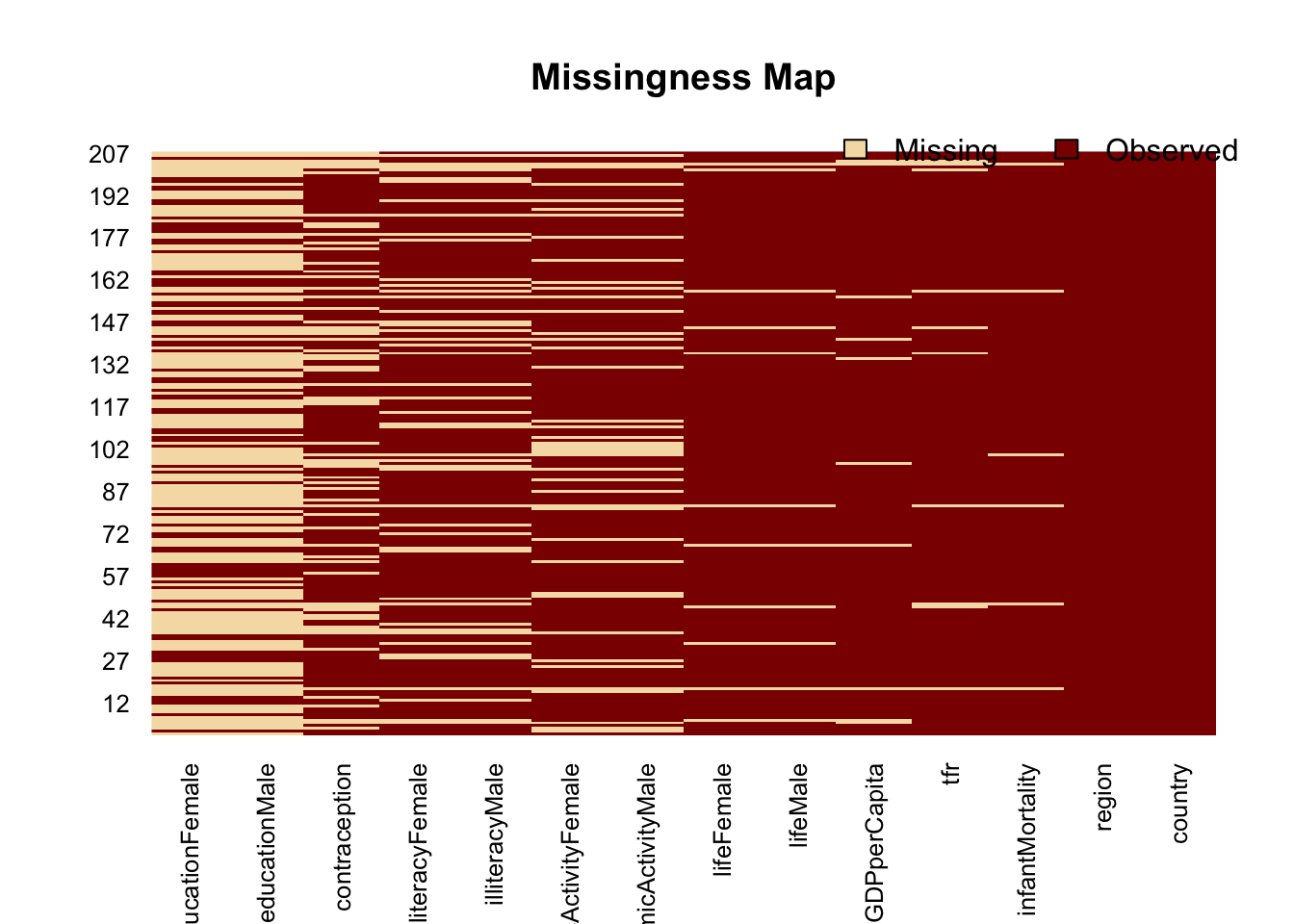
As an aside, and to show you how the combination of dplyr, ggplot occupy a nice spot on the flexibility / amount of code frontier,
UN_miss_mat <-
  mutate(UN, n = row_number()) %>%
  gather(variable, value, - n) %>%
  mutate(is_na = is.na(value)) %>%
  filter(! variable %in% "country")
ggplot(UN_miss_mat,
       aes(x = reorder(variable, is_na, mean), y = n, fill = is_na)) +
  geom_tile() +
  theme_minimal() +
  coord_flip() +
  # this manually sets the colors of the plot; guide = FALSE removes the legend
  scale_fill_manual(values = c("black", NA), guide = FALSE) +
  xlab("") + ylab("Observation number")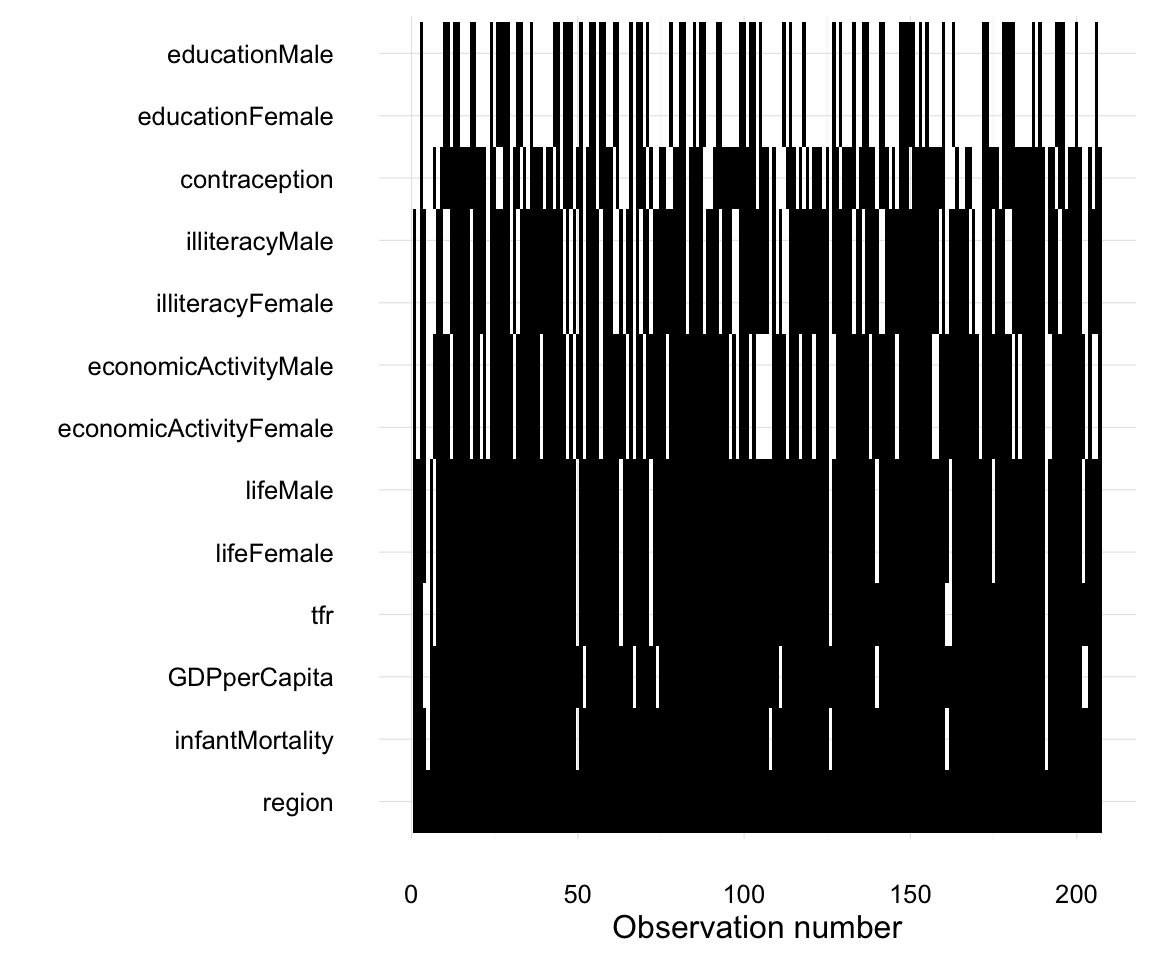
Other tools for visualization missingness are in the VIM package.
Considering that analyses that we will run, with infantMortality, educationFemale, contraception, GDPperCapita. What is the level of missingness if we keep only observations will non-missing values in all the variables? Although the original data has observations for 207 countries, 145 (70%) of them have a missing value for at least one of those variables.
UN %>%
  mutate(n = row_number()) %>%
  select(n, infantMortality, educationFemale, contraception, GDPperCapita) %>%
  gather(variable, value, - n) %>%
  group_by(n) %>%
  summarize(any_missing = any(is.na(value))) %>%
  summarise(total = length(n), total_miss = sum(any_missing),
            miss_frac = total_miss / total)
## Source: local data frame [1 x 3]
##
## total total_miss miss_frac
## (int) (int) (dbl)
## 1 207 145 0.7004831Models
The model we would like to estimate is to regress Infant Mortality on log GDP, contraception and Female Education.
Listwise deletion
We will only use rows for which all the variables used in the model are non-missing. This is what lm() does by default when it encounters missing values.
mod_listwise <-
  lm(infantMortality ~ log(GDPperCapita) + contraception + educationFemale,
     data = UN)
summary(mod_listwise)
##
## Call:
## lm(formula = infantMortality ~ log(GDPperCapita) + contraception +
## educationFemale, data = UN)
##
## Residuals:
## Min 1Q Median 3Q Max
## -47.251 -11.145 0.634 7.925 66.125
##
## Coefficients:
## Estimate Std. Error t value Pr(>|t|)
## (Intercept) 148.245 11.913 12.444 <2e-16 ***
## log(GDPperCapita) -7.580 2.365 -3.205 0.0022 **
## contraception -46.114 17.399 -2.650 0.0103 *
## educationFemale -2.491 1.386 -1.798 0.0775 .
## ---
## Signif. codes: 0 '***' 0.001 '**' 0.01 '*' 0.05 '.' 0.1 ' ' 1
##
## Residual standard error: 17.9 on 58 degrees of freedom
## (145 observations deleted due to missingness)
## Multiple R-squared: 0.7466, Adjusted R-squared: 0.7335
## F-statistic: 56.97 on 3 and 58 DF, p-value: < 2.2e-16Indicator Variables for Missing Values
For each variable, we will add a dummy variable that is equal 1 if that variable is missing and 0 if not. Then for each variable we will replace its missing values with 0 (or its mean). To assist in that, we will define the function fill_na which fills in missing values in x with whatever value is given in fill.
fill_na <- function(x, fill = 0) {
  x[is.na(x)] <- fill
  x
}
Now we generate a new dataset with those dummy variables and with the missing values replaced by their means.
UN_with_dummies <-
  UN %>%
  mutate(GDPperCapita_na = as.integer(is.na(GDPperCapita)),
         GDPperCapita = fill_na(GDPperCapita, mean(GDPperCapita, na.rm = TRUE)),
         contraception_na = as.integer(is.na(contraception)),
         contraception = fill_na(contraception, mean(contraception, na.rm = TRUE)),
         educationFemale_na = as.integer(is.na(educationFemale)),
         educationFemale = fill_na(educationFemale, mean(educationFemale, na.rm = TRUE)))
mod_dummies <- lm(infantMortality ~ log(GDPperCapita) + GDPperCapita_na + contraception +
     contraception_na + educationFemale + educationFemale, data = UN_with_dummies)
mod_dummies
##
## Call:
## lm(formula = infantMortality ~ log(GDPperCapita) + GDPperCapita_na +
## contraception + contraception_na + educationFemale + educationFemale,
## data = UN_with_dummies)
##
## Coefficients:
## (Intercept) log(GDPperCapita) GDPperCapita_na
## 166.4830 -12.5506 3.7953
## contraception contraception_na educationFemale
## -55.0697 3.5130 -0.4682Unconditional Mean Imputation
Another ad hoc method is to replace missing values with their means. Since we filled in the missing values in UN_with_dummies with the mean values, we will use that, but not include the dummy variables.
These bivariate plots illustrate how unconditional imputation means work, and give an indication of how they will affect results.
ggplot(filter(UN_with_dummies, !is.na(infantMortality),
              !is.na(educationFemale)),
       aes(y = infantMortality, x = educationFemale,
           colour = as.factor(educationFemale_na))) +
  geom_point() +
  scale_colour_discrete("Imputed") +
  theme_local()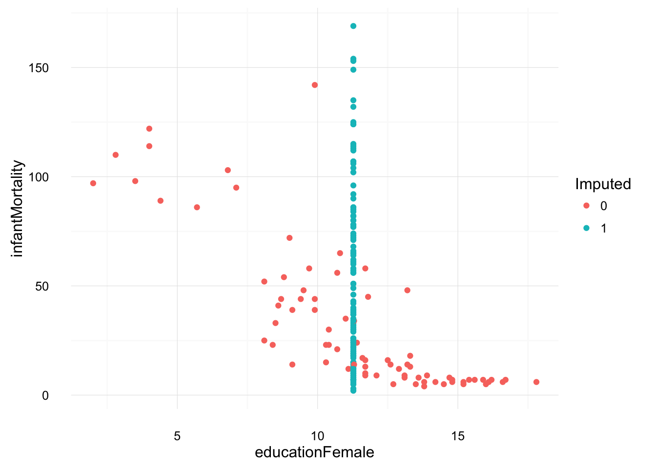
ggplot(na.omit(select(UN_with_dummies, infantMortality,
                      contraception, contraception_na)),
       aes(y = infantMortality, x = contraception,
           colour = as.factor(contraception_na))) +
  geom_point() +
  scale_colour_discrete("Imputed") +
  theme_local()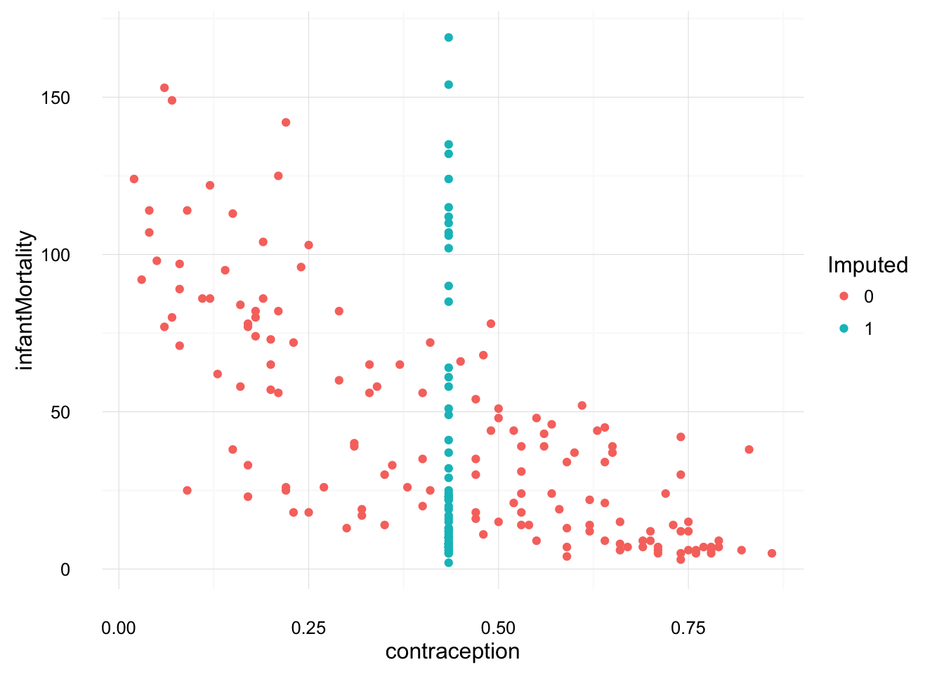
mod_means <- lm(infantMortality ~ log(GDPperCapita) + contraception +
      educationFemale, data = UN_with_dummies)
mod_means
##
## Call:
## lm(formula = infantMortality ~ log(GDPperCapita) + contraception +
## educationFemale, data = UN_with_dummies)
##
## Coefficients:
## (Intercept) log(GDPperCapita) contraception
## 166.5511 -12.2072 -56.1593
## educationFemale
## -0.5595Multiple Imputation
Our preferred method is multiple imputation. For multiple imputation we will use the implementation in Amelia.1 Multiple imputation works by creates \(m\) datasets with the missing values filled in with imputations. The analyst then runs the analysis on each of the datasets, and there are (fairly easy) methods to combine the estimates and standard errors from the individual analyses into an overall point estimate and standard error. The function amelia creates these imputations.
m = 5is the number of observations. Usually5 - 10are sufficient. See Fox, p. 564.ameliamodels the distribution of the data as multivariate normal so it is useful to transform the data to make it more normal. Use the argumentslogsto indicate variables to log transform, andlgstcto logistic transform variables.- Additionally, you need to tell
ameliawhich variables are nominal (noms =) so it creates dummy variables; and which variables are id variables (idvars =) so it can ignore them in the imputation process, but still include them in the final datasets.
UN_mi <-
  amelia(data.frame(UN),
         m = 5,
         logs = c("GDPperCapita"),
         lgstc = c("economicActivityMale", "economicActivityFemale",
                   "illiteracyMale", "illiteracyFemale", "contraception"),
         noms = c("region"),
         idvars = "country")
Note I had to use data.frame because at the moment amelia has bugs when using dplyr data_frame objects.
Note several things about the imputation process.
First, the number of imputations is small, m = 5. There is not much improvement in the performance of multiple imputation from using many imputations. Usually 5–10 is more than sufficient. See Fox, p. 564.
Second, we use the dependent variable as well as variables not used in the regression in the imputation. (Fox, p. 567) This is not an issue. Concerns like endogeneity and multicollinearity are not concerns in this context; we are not interested in estimating unbiased coefficients. We are concerned with predicting the values of these variables.
The multiple imputation process has created m = 5 separate datasets, which are stored as a list of data frames in the imputations element of the object:
str(UN_mi$imputations)Each of these datasets is complete, meaning it has no missing observations. But for values which were missing in the original data, they are filled with different imputations. For example, compare this subset in the orginal data and two imputations.
countries <- c("Afghanistan", "Angola", "Algeria", "Antigua")
UN %>% filter(country %in% countries) %>% select(country, contraception)
## Source: local data frame [4 x 2]
##
## country contraception
## (chr) (dbl)
## 1 Afghanistan NA
## 2 Algeria 0.52
## 3 Angola NA
## 4 Antigua 0.53UN_mi$imputations[[1]] %>% filter(country %in% countries) %>% select(country, contraception)## country contraception
## 1 Afghanistan 0.07640913
## 2 Algeria 0.52000000
## 3 Angola 0.14690295
## 4 Antigua 0.53000000UN_mi$imputations[[2]] %>% filter(country %in% countries) %>% select(country, contraception)## country contraception
## 1 Afghanistan 0.06033049
## 2 Algeria 0.52000000
## 3 Angola 0.28073275
## 4 Antigua 0.53000000The following creates plots of each variable, overplotting the values from each imputation against the observation number. Points which are black were observed in the original data; points which are gray are imputed.
all_imputations <-
  data_frame(i = seq_len(UN_mi$m)) %>%
    rowwise() %>%
    do({
      mutate(UN_mi$imputations[[.$i]],
             .obsnum = row_number(),
             .imputation = .$i)
    })

imputation_plot <- function(yvar) {
  ggplot(all_imputations, aes_string(x = ".obsnum",
                                     y = yvar)) +
  geom_point(alpha = 0.2) +
  theme_minimal() +
  xlab("Observation number") +
  theme_local()
}

imputation_plot("educationFemale")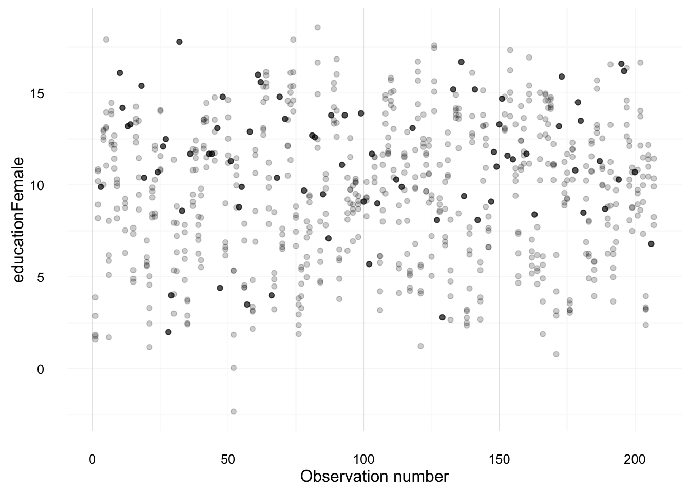
imputation_plot("contraception")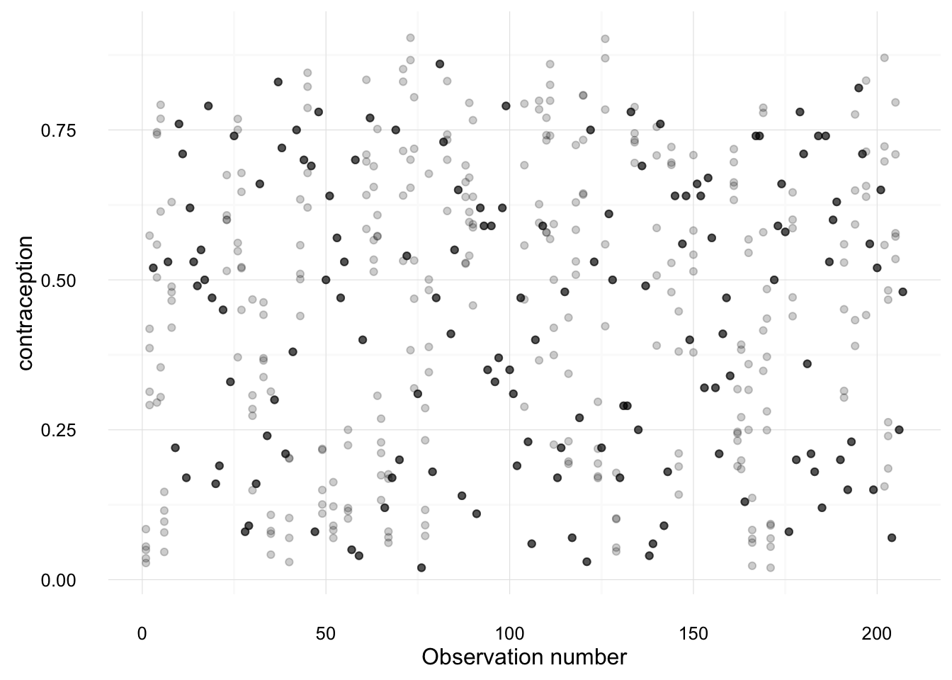
imputation_plot("log(GDPperCapita)")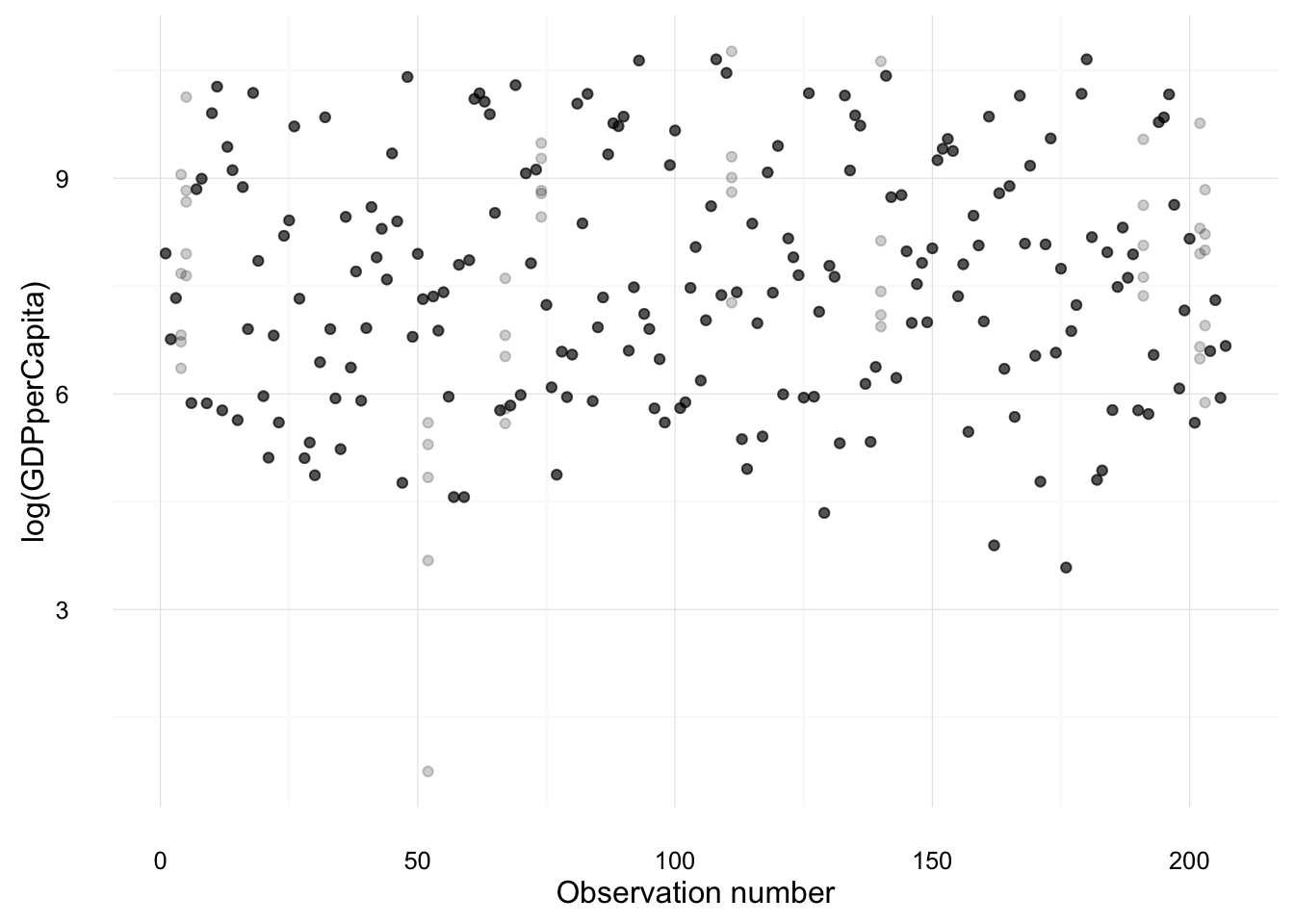
Let’s see how one of these imputed datasets looks and compare the imputed and non-imputed values as an informal way of judging its plausibility.
ggplot(UN_mi$imputations[[1]] %>%
         mutate(missing = UN_mi$missMatrix[ , "educationFemale"]),
       aes(x = educationFemale, y = infantMortality, colour = missing)) +
  geom_point() +
  theme_local()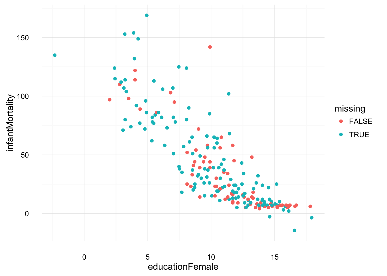
ggplot(UN_mi$imputations[[1]] %>%
         mutate(missing = UN_mi$missMatrix[ , "contraception"]),
       aes(x = contraception, y = infantMortality, colour = missing)) +
  geom_point() +
  theme_local()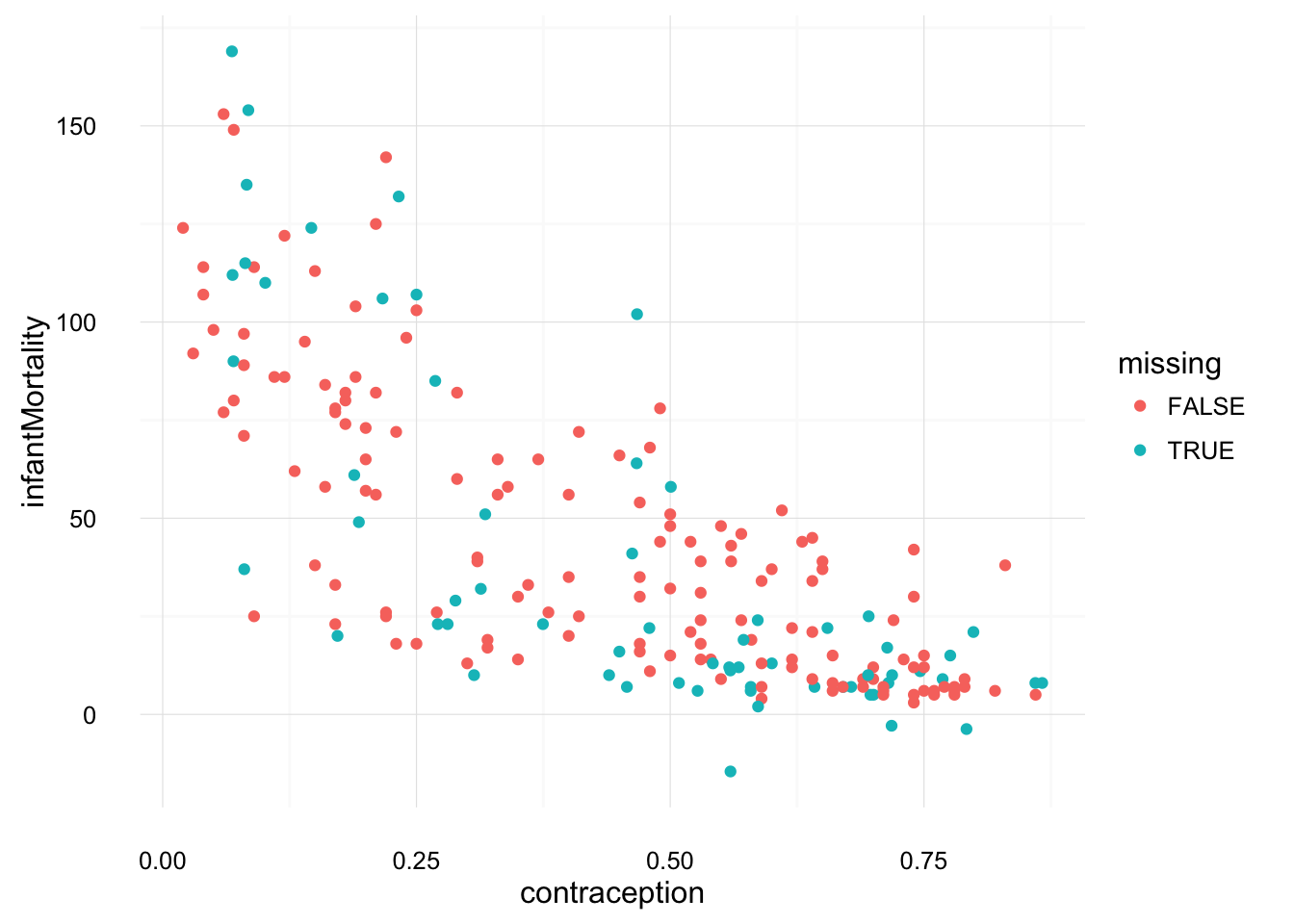
These look much more plausible than those of the unconditionally imputed mean.
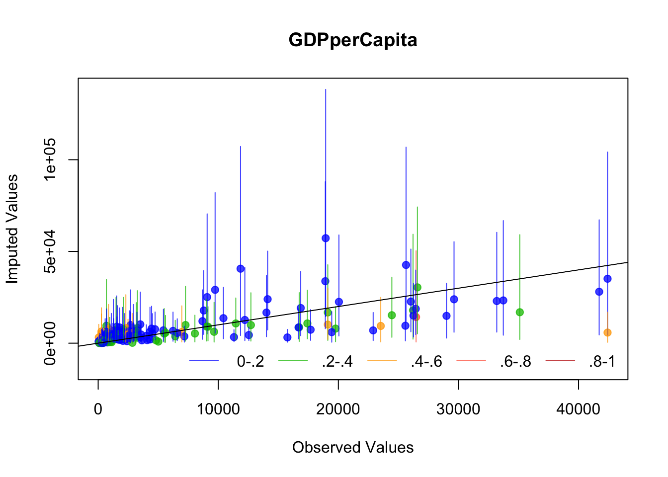
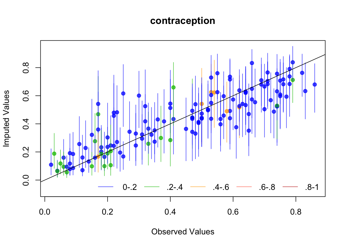
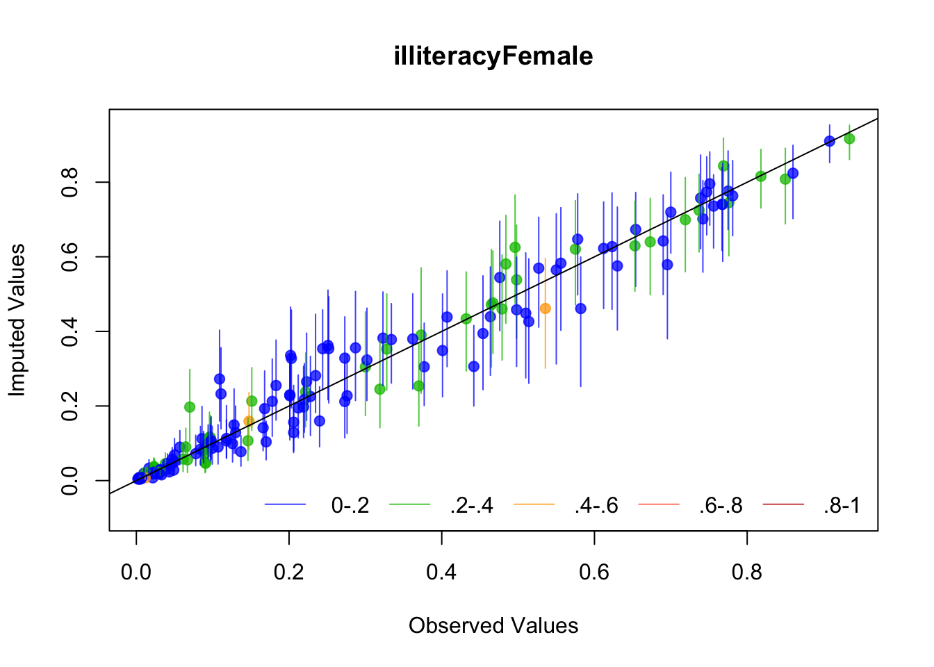
The plots we just made suggest Amelia is working well, but let’s look at a couple of diagnostics that Amelia suggests: The first is to drop each observation of a variable, impute it, and plot the values against the original values. If the imputed values resemble the original values, then the imputation procedure has worked well.
Amelia suggests several diagnostics for evaluating The first is “overimputation”. This is similar to leave-one-out cross validation. Each observation is removed and treated as a missing value to be imputated. Amelia plots 90% confidence intervals for each observation against the true values. If the imputation is reasonable, then these confidence intervals should have 90% coverage of the true value. The following code runs the overimputation diagnostic for the variables of interest (the ones that will be used in the regression). The overimputation diagnostics do not suggest any issues with the imputation of these variables.
for (var in c("GDPperCapita", "contraception", "illiteracyFemale")) {
  overimpute(UN_mi, var, main = var)
}
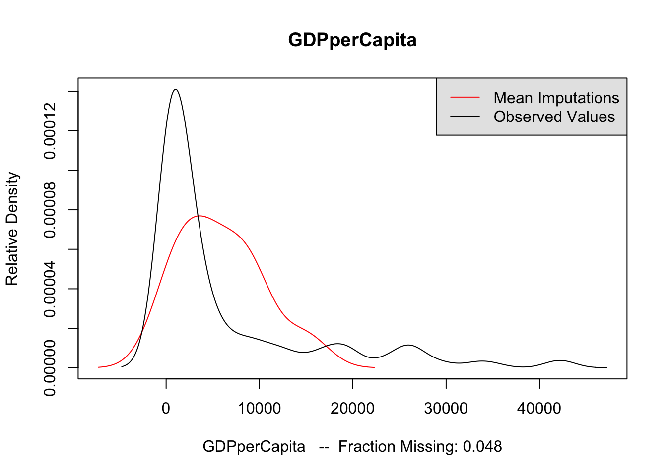
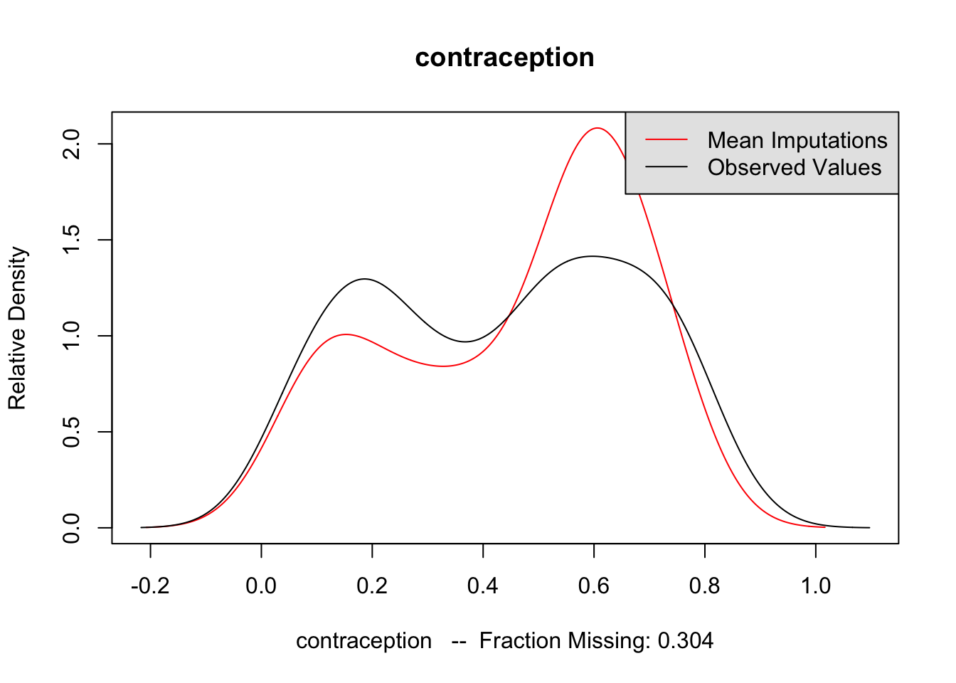
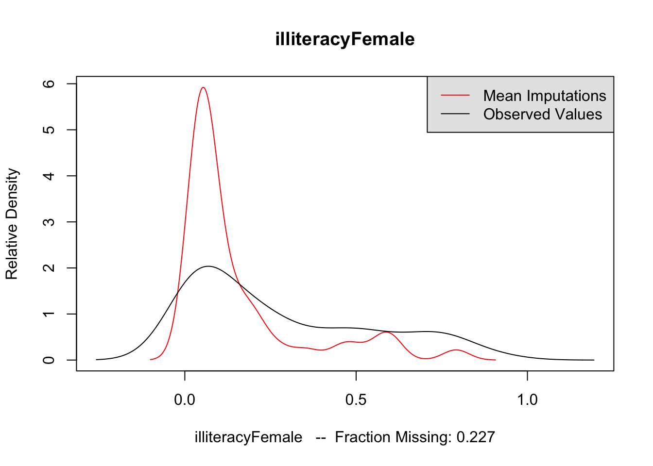
The second method is to plot the marginal density of the imputed values against observed values. If these appear too different, then there may be issues with imputation. However, there is no particular criteria for what is too different, and there may be reasons why these distributions diverge; see the Amelia vignette for an example of what would be a big difference. But if these distributions are different, then you should revisit the data to see whether imputation makes sense. The following code performs this for each variable of interest. The plots do not suggest any differences to be concerned about.
for (var in c("GDPperCapita", "contraception", "illiteracyFemale")) {
  compare.density(UN_mi, var, main = var)
}
Now that we are satisfied that the imputations are reasonable, we run the analysis on each of the imputated datasets. The following code runs the regression on each imputed dataset saving the coefficients to b_out, and the standard errors of the coefficients to se_out. These are originally saved to a list, but rbind converts it to a matrix with each imputations as rows and coefficients as columns.
Now estimate the model using each imputed dataset. We save the results to b_out and se_out.
b_out <- list()
se_out <- list()
for (i in seq_along(UN_mi$imputations)) {
  mod <- lm(infantMortality ~ log(GDPperCapita) + contraception + educationFemale, data = UN_mi$imputations[[i]])
  b_out[[i]] <- coef(mod)
  se_out[[i]] <- sqrt(diag(vcov(mod)))
}
b_out <- do.call(rbind, b_out)
se_out <- do.call(rbind, se_out)
As described in Fox or Gelman, the coefficients from the imputations can be combined to calculate a single point estimate and standard error. The function mi.meld does this, and returns a list with point estimates in the element q.mi and standard errors in se.mi:
mod_mi_res <- mi.meld(q = b_out, se = se_out)
mod_mi_res
## $q.mi
## (Intercept) log(GDPperCapita) contraception educationFemale
## [1,] 134.5969 -2.699894 -45.31222 -5.023085
##
## $se.mi
## (Intercept) log(GDPperCapita) contraception educationFemale
## [1,] 13.43238 3.431773 14.32526 1.894144Model Comparison
Now that we’ve estimated this model using various methods to handle missing data, let’s compare the results. First, we combine these into a single dataset. For the results returned by Amelia, since there is no tidy function defined for Amelia objects we need to manually create a data frame consistent with those returned by tidy.
model_comp <-
  bind_rows(tidy(mod_listwise) %>%
              mutate(model = "listwise"),
            tidy(mod_dummies) %>%
              mutate(model = "dummies"),
            tidy(mod_means) %>%
              mutate(model = "means"),
            data_frame(term = colnames(mod_mi_res$q.mi),
                       estimate = as.numeric(mod_mi_res$q.mi),
                       std.error = as.numeric(mod_mi_res$se.mi),
                       model = "mi"))
plot_mi_models <- function(data, variable) {
ggplot(data %>%
filter(term %in% variable),
aes(x = model, y = estimate,
ymin = estimate - 2 * std.error,
ymax = estimate + 2 * std.error)) +
geom_pointrange() +
geom_hline(yintercept = 0, colour = "red", alpha = 0.2) +
coord_flip() +
theme_minimal()
}
plot_mi_models(model_comp, "log(GDPperCapita)")
plot_mi_models(model_comp, "contraception")
plot_mi_models(model_comp, "educationFemale")
These plots show that the various methods produce different answers both in terms of point-estimates and standard errors. Though, we would have to use simulations to determine why the imputation methods are better than the alternatives.
There are several other R packages that do multiple imputation. For example, mice and mi, which use a different method, called chained equations. We will use Amelia because it is stable, works well, and since it is written by Gary King, it is the one that most political scientists are familiar with.↩